Introduction
Context
Artificial intelligence (AI) is increasingly prevalent in our daily lives, revolutionizing not only personal gadgets but also transforming our modes of transportation. Analogous to the rise of electric vehicles, fully autonomous vehicles undoubtedly represent the future of the transportation industry. Among the multifaceted applications of AI in autonomous driving, one pivotal function is the real-time analysis of the vehicle’s surrounding environment, including signals, traffic, and anomalies.
This project is part of the Ecotrain project, which aims to develop an AI capable of interpreting image content captured by a camera at the front of the train. The Ecotrain project stands as a pioneering initiative aimed at redefining the landscape of public transportation through the integration of autonomous technology into the rail system. Spearheaded by a consortium of industry leaders, research institutions, and technology firms, the project’s ambition is to launch France’s inaugural autonomous rail shuttle service by 2026. By equipping the autonomous shuttle with advanced image interpretation capabilities, the project seeks to navigate the complex dynamics of rail travel, from signal recognition and traffic analysis to anomaly detection. The AI’s ability to process and understand live video frames feeds will be instrumental in ensuring the shuttle’s safe operation, paving the way for a new era of smart, autonomous public transport systems.
The Ecotrain project is an innovative venture that aims to revolutionize the public transportation landscape by developing a train that is not only autonomous but also 100% electric. Ecotrain lines aim to be non-invasive in terms of equipment and terrain alteration, emphasizing the project’s commitment to sustainability and environmental conservation. By leveraging lightweight, electric trains and revitalizing unused railways, Ecotrain seeks to offer a green, efficient alternative to current transportation options, reducing carbon emissions and reliance on fossil fuels.This autonomy places the entire responsibility for safety and security on the train, necessitating a comprehensive array of sensors and technologies to accurately perceive and interpret the environment. Such a setup allows the train to navigate through complex rail networks safely, making real-time decisions based on the data gathered from its surroundings. The integration of advanced image interpretation capabilities is a cornerstone of this project, enabling the autonomous shuttle to recognize signals, analyze traffic, and detect anomalies, ensuring the safe operation of the service.
The role of IMT Nord Europe, where this research project is taking place, in the Ecotrain project underlines the collaborative effort behind this initiative. The institution is involved in developing secure, short-range radio communication solutions, facilitating the safe transmission of information critical to the operation of autonomous trains. Additionally, the team I’m working with in IMT Nord Europe aims to create autonomous technological solutions for sensor data fusion. This work is pivotal in enabling predictive analysis of moving objects’ trajectories, further enhancing the safety and reliability of the autonomous rail shuttle service. Through the combined efforts of industry leaders, research institutions, and technology companies, the Ecotrain project aspires to launch France’s first autonomous rail shuttle service by 2026, setting a new standard for smart, sustainable public transport systems.
Challenges
The central challenge addressed by the Ecotrain project revolves around the development of an advanced AI system capable of intricate environmental analysis in real-time. This system must accurately interpret image content captured by a camera mounted at the front of the train, discerning signals, navigating traffic, and identifying anomalies. The complexity of rail travel dynamics, compounded by the need for immediate and precise decision-making, necessitates an AI with unparalleled image interpretation capabilities. This endeavor not only signifies a leap towards sustainable and efficient rail travel but also encapsulates a commitment to enhancing passenger safety, operational efficiency, and environmental sustainability.
Incorporating scene graphs into this project is essential for enhancing the AI’s ability to assess risks by analyzing the complex environment in real-time. Scene graphs provide a structured representation of the visual scene, identifying objects and their relationships, which is crucial for detecting anomalies and evaluating potential hazards on the rail tracks. This method allows for a deeper understanding of each element’s context within the scene, leading to more accurate and nuanced risk assessments. Utilizing scene graphs bridges the gap between simple object detection and understanding the intricate dynamics of rail environments, ultimately contributing to the safety and efficiency of autonomous rail travel.
Objectives
In this research, the initial focus is on the triplets derived from the scene graph generation models, consisting of subject-relation-object, where each subject and object is associated with its bounding box. We first create a fundamental risk analysis model based on these triplets to demonstrate the feasibility of the overall method. While scene graphs have led to several state-of-the-art models in the areas of automatic image annotation, image mining, and image generation, their utilization for risk analysis in an autonomous driving system remains largely unexplored. The objective is to explore and validate the use of scene graphs in creating a robust framework for real-time risk assessment, ultimately contributing to the success of the Ecotrain project and advancing the safety and reliability of autonomous public transportation systems.
Scene Graph Generation
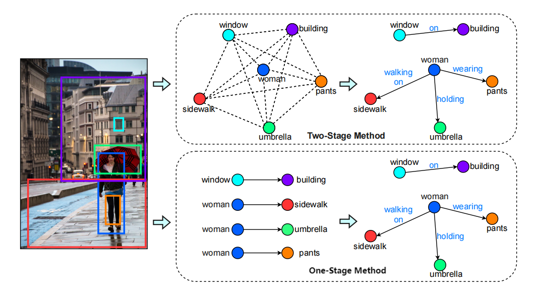
Scene graph generation has become a cornerstone in the field of computer vision, especially for tasks requiring a deep understanding of complex visual scenes. At its core, a scene graph encapsulates the entities within an image and their interrelationships, offering a structured representation that greatly enhances image comprehension. Predominantly, there are two methodologies in scene graph generation: the two-stage and one-stage methods. Numerous one-stage and two-stage methods have been developed thanks to the contributions of researchers in the field. Each approach has its unique mechanisms and applications, contributing differently to the advancement of scene graph research.
Definition
A Scene Graph (SG) is formally defined as a directed graph data structure, described by the tuple SG = (O, R, E), where:
$O = {o_1,…,o_n}$ is the set of objects identified in an image, and $n$ represents the total number of these objects. An individual object $o_i$ is characterized by the tuple $o_i = (c_i, A_i)$, with $c_i$ indicating the object’s category and $A_i$ its attributes.
$R$ represents the relationships established between the nodes, with a specific relationship from the $i$-th to the $j$-th object instance denoted as $r_{i\rightarrow j}$, and $i,j$ belonging to the set ${1,2,…,n}$.
$E \subseteq O \times R \times O$ maps the edges that connect object instance nodes through relationship nodes. Initially, the graph might comprise as many as $n \times (n-1)$ edges. However, edges such as $Edge(o_i, r_{i\rightarrow j}) \in E$ where $o_i$ is classified as ‘background’ or $r_{i\rightarrow j}$ is deemed ‘irrelevant’, are systematically pruned from the graph. This process underscores that for an input image $I$, the Scene Graph Generation (SGG) method yields a scene graph $SG$. This graph includes object instances delineated within the image by bounding boxes, along with the depicted relationships among the object pairs.
The generation process can be succinctly expressed as:
$$SG_{O,R,E}^I = SGG(I)$$
This structured approach to defining a scene graph facilitates a comprehensive understanding of the visual scene, enabling detailed analyses and interpretations based on the detected objects and their interrelationships.
Generation Process
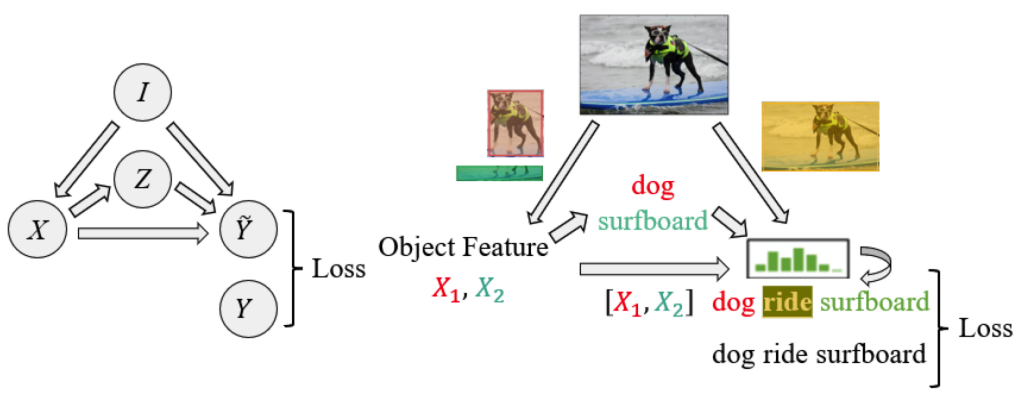
The overarching methodology of Scene Graph Generation (SGG) is depicted in Figure above. This figure is split into two parts for enhanced clarity: Figure left offers a schematic overview of the SGG workflow, whereas Figure right provides a tangible instance of the process. The node $I$ signifies the input image, serving as the foundational element from which the scene graph is constructed. Node $X$ encapsulates the extracted features of the detected objects within the image, acting as a crucial intermediary that bridges raw visual data with semantic understanding. Node $Z$ is tasked with identifying the object’s category, translating the abstract features into recognizable entities. The predictive node $\hat{Y}$ is central to deducing the relationship categories and assembling the corresponding triplet $\langle s, p, o \rangle$. It employs a sophisticated fusion function that integrates inputs from the object features, categories, and predicted relationships to yield the logits that underpin the final scene graph predictions. Lastly, node $Y$ denotes the actual labels of the triplets, providing a benchmark against which the accuracy of the generated scene graph can be measured. The explanation of the corresponding step is as follows:
Extraction of Object Features ($I \rightarrow X$)}: The extraction of object features and bounding boxes from an input image $I$ is typically facilitated by a pretrained Faster R-CNN model. This method yields a collection of bounding boxes $B = {b_i | i = 1, …, m}$ alongside their corresponding feature representations $X = {x_i | i = 1, …, m}$, encapsulated as:
$$
Input: {I} \Rightarrow Output: {x_i | i = 1, …, m}.
$$
This step crucially captures the visual context for each detected object.Classification of Objects ($X \rightarrow Z$): At this juncture, the extracted features are translated into object classifications. The process can be succinctly defined as:
$$
Input: {x_i} \Rightarrow Output: {z_i, z_i \in O}, i = 1, …, m.
$$Input of Object Classes for SGG ($Z \rightarrow \widetilde{Y}$): This step involves leveraging the labels of paired objects $(z_i, z_j)$ to forecast the predicates $\widetilde{y}$ between them, using a combined embedding layer $M$. The operation is outlined as:
$$
Input: {(z_i, z_j)} \overset{M}{\Longrightarrow} Output: {\widetilde{y}_{ij}}, i \neq j; i,j = 1, …, m.
$$Input of Object Features for SGG ($X \rightarrow \widetilde{Y}$): Here, the combined features of object pairs $[x_i, x_j]$ are used to anticipate the predicates that define their relationship. This procedure is expressed as:
$$
Input: {[x_i, x_j]} \Rightarrow Output: {\widetilde{y}_{ij}}, i \neq j; i,j = 1, …, m.
$$
This delineation underscores the sequential and interconnected nature of the SGG process, from initial image input through to the generation of a comprehensive scene graph that articulately describes the interplay of objects within the visual scene.
Two-Stage Method
The two-stage method is a traditional approach where the first stage focuses on detecting objects within an image, creating entity proposals. The second stage then identifies the relationships between these proposed entities. This method is characterized by its thoroughness in capturing the dense relationships among entities, relying on the initial comprehensive object detection to ensure that no potential interaction is overlooked. However, this robustness comes with a cost: a significant computational load and a tendency towards generating overly dense graphs that may include redundant or irrelevant relationships. Despite these challenges, two-stage methods have been instrumental in pushing forward the boundaries of scene graph generation, providing detailed scene interpretations that facilitate tasks such as image captioning and visual question answering.
One-Stage Method
Emerging as a response to the computational intensity and complexity of two-stage methods, the one-stage method simplifies the scene graph generation process. It bypasses the distinct object detection phase, directly predicting the relationships between entity pairs within the image. This streamlined approach aims to produce a sparse scene graph that focuses on the most salient interactions, leveraging visual appearances without the intermediary step of object proposal generation. The one-stage method’s efficiency and directness make it particularly suited for applications requiring faster processing times and simplified scene graphs that capture essential interactions. While the one-stage method is celebrated for its efficiency and the simplification it brings to the scene graph generation process, it is not without its limitations. This approach may sometimes overlook subtle or less prominent relationships due to its focus on directly predicting relationships without the detailed context that object detection provides. Consequently, the resulting scene graphs might lack the depth and comprehensive understanding of the scene that two-stage methods offer. Additionally, the direct prediction of relationships can lead to challenges in distinguishing between closely related categories or in cases where visual cues alone are insufficient for accurate relationship inference.
Models used in this Study
In the pursuit of advancing scene graph generation for autonomous train navigation, I employed two distinct models, each contributing uniquely to the project’s objectives. By harnessing the power of their advanced scene graph generation capabilities, we lay the foundation for my subsequent risk analysis, setting the stage for a nuanced understanding of the dynamic scenarios encountered in traffic.
The two models, both pretrained on the Visual Genome dataset, to generate relational triplets and corresponding bounding boxes for subjects and objects within the scene. And these two pretrained models, a cornerstone of my risk analysis framework, both of them are trained to recognise the same wide range of entities and relationships. This setup is critical to fully understand the scene in the context of the railway environment and to compare their performance for the subsequent risk analysis task. A complete list of detected entities classes is available in Appendix A, and relationship classes are listed in Appendix B.
Below, we delve into the specifics of these models, highlighting their methodologies and the roles they play in enhancing the system’s capability to analyze and understand complex visual scenes.
The RelTR Model
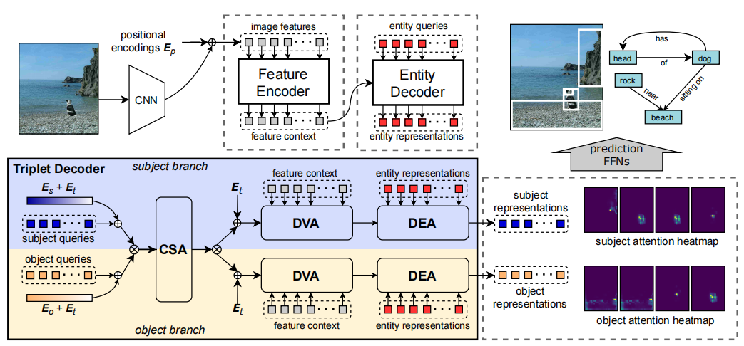
In the ambit of real-time environmental analysis for autonomous transportation, the RelTR model emerges as a transformative approach. Distinct from conventional multi-stage methods, RelTR’s architecture integrates scene graph generation into a single-stage process. This integration is pivotal for my project, given the necessity for rapid and accurate interpretation of dynamic surroundings. The model’s encoder leverages visual inputs to contextually map the environment, while the decoder predicts inter-object relationships, forming a sparse scene graph. Such a graph delineates the relational structure between entities, essential for autonomous trains to comprehend and react to complex scenarios.
The RelTR model is underpinned by a robust technical architecture that is designed to optimize scene graph generation for real-time applications. Its single-stage framework is a departure from the traditional multi-stage systems, streamlining the process of understanding visual environments. The encoder in RelTR employs a transformer-based mechanism that processes the entire image as a sequence, allowing the model to capture global context effectively. The decoder then applies an attention mechanism that enables the model to focus on relevant parts of the image to predict relationships between entities accurately. This efficient architecture facilitates quick and precise identification of objects and their interrelations, which is crucial for the real-time decision-making processes in autonomous train navigation. The technical sophistication of RelTR ensures that it can be seamlessly integrated into the autonomous navigation system, providing immediate environmental interpretations essential for the operation of autonomous trains.
The MOTIFS-SGDet-TDE Model
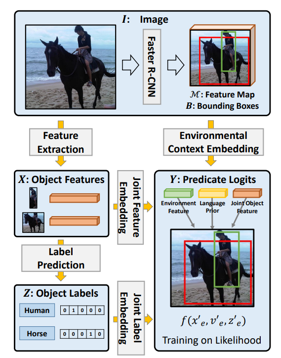
Contrasting with RelTR’s one-stage approach, the MOTIFS-SGDet-TDE model exemplifies the two-stage methodology’s strengths. It focuses on leveraging motifs—common patterns found within scene graphs—to enhance relationship detection between entities. See in Figure above, the model first applies a Faster R-CNN to the input image (I) to generate a feature map (M) and detect bounding boxes (B). Next, feature extraction is performed to produce object features (X), which are then combined with environmental context embeddings. This joint feature embedding is used to predict predicate logits (Y). The object features and embeddings are also used for label prediction, producing object labels (Z). The model uses statistical motifs from scene graphs for refined relationship detection, capturing the nuanced interplay of elements within the scene. Its effectiveness stems from its sophisticated mechanism that takes advantage of statistical regularities in scene graph data, thereby improving the accuracy of relationship prediction. While it embraces the computational complexity typical of two-stage methods, this model stands out for its ability to deepen scene understanding through the exploitation of recurring relational motifs.
What sets the MOTIFS-SGDet-TDE model apart is not just its reliance on motifs but also its comprehensive framework, which permits a nuanced understanding of the visual scene. This depth of scene comprehension is crucial for applications like mys, where discerning intricate relationships directly influences decision-making processes. Despite the inherent computational demand, characteristic of two-stage models, its efficiency in mining relational motifs facilitates a richer, more detailed scene graph output, thereby enhancing the AI’s environmental analysis capabilities.
A Fundamental Risk Analysis Model
We explore the development of a foundational risk analysis model. It elaborates on the methodology of assigning risk scores to these entities and relationships, analyzing bounding box dimensions, and visualizing potential hazards through heatmaps. This comprehensive approach encapsulates the model’s jmyney from conceptualization to integration, highlighting its significance in enhancing the safety and reliability of autonomous train systems.
Before delving into the specific metrics and performance assessments of this fundamental risk analysis model, it is pertinent to acknowledge the gap in the dataset landscape. Currently, there is an absence of a rail driving dataset with appropriately annotated formats tailored for the RelTR and MOTIFS-SGDet-TDE models. In response to this, my efforts are directed towards leveraging the models pre-trained on the Visual Genome (VG) dataset. The VG dataset, while primarily focused on urban environments, provides a proxy for inference that is moderately analogous to the rail context. We are actively investigating the transferability of knowledge from this urban-centric dataset to the domain of rail driving. This includes the modification of learned rules and heuristics to suit the unique characteristics and requirements of the rail environment. Such an endeavor is not without its challenges; however, it is a crucial step towards creating a bespoke solution that can accurately comprehend and navigate the intricacies of rail systems.
Risk Score Assignment
The quantification of danger in the context of autonomous driving is pivotal to ensuring safety and reliability. There are also other related publications that also define identical criteria for autonomous driving.
The assignment of risk scores in the model is a meticulously crafted process, central to transforming visual data into a coherent risk assessment framework. Each entity and relationship identified by the model is assigned a numerical risk score, reflecting its potential hazard in the context of railway environments. These scores range from 0 to 10, offering a granular spectrum of risk levels where 0 represents no risk and 10 signifies the highest possible risk. This scoring system is not arbitrary but is based on a comprehensive understanding of various elements typically encountered along rail routes. Objects like vehicles, pedestrians, and infrastructural elements, as well as their interactions, are all evaluated for their potential to impact the safety of the autonomous train. The assignment is guided by predefined criteria, ensuring consistency and reliability in the risk evaluation.
For instance, static objects might be assigned lower scores compared to dynamic entities like moving vehicles, which pose a greater risk. Similarly, relationships indicating proximity to the railway tracks would garner higher scores due to their immediate relevance to train operation. In refining the model, relationships that involve entities with a score of 0 are filtered. This is based on the premise that certain objects and their associated relationships have negligible impact on the operation and safety of the train. For example, we don’t care about the relationship ‘banana near car’. This filtering step ensures that the risk assessment remains focused on significant hazards. The process of assigning risk scores to each detected entity involves calculating the mean score of the tuples to which the entity belongs. For instance, consider the tuple “person near car.” In this scenario, “person” is assigned a risk score of 5, the relationship “near” has a score of 8, and “car” has a score of 7. Here what needs to be clarified is that the specific risk values assigned to entities are subjectively determined based on experience and according to the basic rules introduced above. Consequently, the average risk score assigned to the bounding box areas of both “person” and “car” in this tuple would be calculated as follows:
$$ \frac{5 (\text{person}) + 8 (\text{near}) + 7 (\text{car})}{3} = 6.67 $$
This average score represents the combined risk of the entities and their relationship within the context of the scene, providing a balanced assessment of the potential hazards each entity poses in conjunction with others. Importantly, the global score for the scene is determined by the highest mean score among all detected relationships. This approach ensures that the most significant risk within a scene sets the benchmark for the overall safety assessment, allowing for focused attention on the most critical areas of concern.
This scoring system transforms the relationship data into a valuable tool for real-time decision-making, enabling the autonomous system to prioritize responses based on the level of risk posed by various elements in its environment.
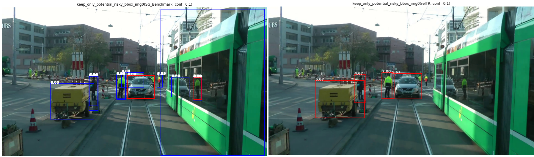
Bounding Box Analysis
The bounding box analysis process involves evaluating the spatial dimensions and locations of detected subjects and objects within the visual frame. By analyzing these bounding boxes, the model gains insights into the physical positioning and potential interactions of different elements in the train’s environment. This analysis is not just about identifying objects but understanding their contextual relevance based on size and location. For instance, larger bounding boxes or those overlapping with the train’s trajectory might indicate more immediate or significant risks, necessitating a higher risk score. This approach allows for a more nuanced understanding of each scene, where the physical dynamics of the objects are as crucial as their identities, feeding into a comprehensive risk assessment strategy tailored for autonomous train operation.
In practice, for this fundamental risk analysis model, we have only retained the smaller bounding boxes. Generally, smaller objects are likely to have a higher risk factor, such as pedestrians compared to cars, and cars compared to trucks.
Scene Risk Heatmaps Generation
This part covers the steps involved in creating a heatmap representation and explains how the risk scores were visually represented in the context of the train’s environment. The heatmap overlaid on the train’s front camera view can provide a clear and intuitive representation of potential risks.
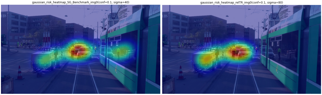
Gaussian Heatmap Generation
The generation of the Gaussian heatmap is a critical aspect of visualizing the potential risks in the train’s environment. This heatmap utilizes the potential risk entities identified from the previous section step, providing a visual overlay on the train’s frontal camera view. The Gaussian heatmap is particularly effective in representing the spatial distribution of risks, offering an intuitive understanding of areas that require immediate attention.
- Initial Setup: The process begins with the creation of an empty heatmap matrix, matching the dimensions of the train’s frontal camera view. This matrix serves as the foundation for accumulating risk scores.
- Risk Score Integration: For each potential risk entity, it has its risk score and bounding box. These scores are then plotted onto the heatmap matrix at the location of each entity. The central point of the bounding box is used as the anchor for the heatmap and the plotting.
- Gaussian Distribution Application: To represent the risk scores spatially and intuitively, a Gaussian filter is applied to each point where a risk score is plotted. This step spreads the risk score outward from its central point, creating a blurred effect that intuitively represents the potential risk radius. The intensity of the blur (controlled by the $\sigma$ value of the Gaussian filter) correlates to the magnitude of the risk, with higher scores spreading further.
- Normalization and Visualization: The resulting heatmap is then normalized by the max value of risk score which is 10 in our case to ensure that the highest risk scores correspond to the brightest intensities on the heatmap and the comparability between different senarios. This normalization makes the heatmap easier to interpret and aligns with standard heatmap representations. The heatmap is then overlaid on top of the camera view, with varying color intensities representing different risk levels.
This Gaussian heatmap thus provides a dynamic and continuous representation of risk in the train’s immediate vicinity, enabling operators or autonomous systems to quickly identify and respond to potential hazards.
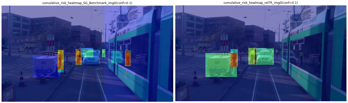
Cumulative Heatmap Generation
The cumulative heatmap generation is an advanced approach designed to visually represent the aggregated risk across overlapping entities in the train’s field of view. This methodology is distinct from the Gaussian heatmap as it focuses on the cumulative aspect of risk in areas where multiple entities or relationships overlap, reflecting a more nuanced understanding of complex scenarios.
- Initial Setup: Similar to the Gaussian heatmap, a matrix matching the camera view’s dimensions is created. However, this matrix is specifically designed to accumulate risk scores from overlapping entities.
- Plotting and Accumulation: The computed risk scores are plotted onto the heatmap at the respective locations of each entity. When bounding boxes of different entities overlap, their risk scores are summed up in the overlapping region. This cumulative effect highlights areas with multiple potential hazards, providing a clearer picture of compounded risks.
- Normalization and Visualization: The final step involves normalizing the heatmap to ensure a consistent representation of risk levels. This normalized heatmap is then overlaid on the train’s camera view. Different color intensities in the heatmap correspond to varying levels of cumulative risk, offering an immediate visual cue to the most hazardous areas.
This cumulative heatmap thus serves as an another essential method in the risk assessment model, particularly in scenarios where multiple risks coexist and interact, necessitating a comprehensive and layered approach to hazard evaluation.
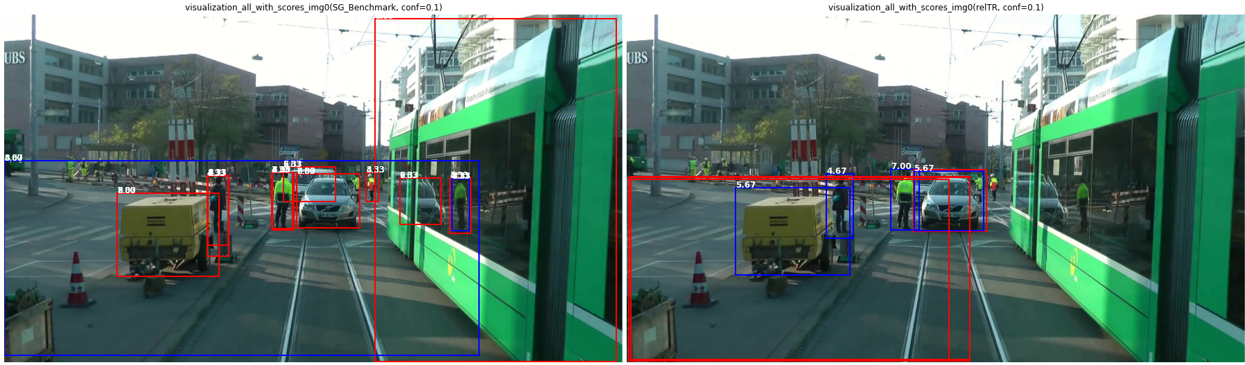
Comparative Performance Analysis of the Two Models
In previous Figures, we observe that both the two-stage model MOTIFS-SGDet-TDE and the one-stage model RelTR yield impressive results in object detection and risk heatmap generation, even with the application of a basic risk analysis model. My point of interest, however, lies in determining which model performs better, as such an analysis holds substantial value for my project.
My fundamental risk analysis model currently does not account for factors such as weather or light conditions, yet it still allows us to make preliminary assessments of general risk accuracy. Given that both pretrained models are based on the same VG dataset and the resulting risk analysis is derived from my uniform fundamental risk analysis model, the context remains consistent. This consistency ensures that their performances are comparable and meaningful within the specific context of my scientific inquiry.
Dataset
For this comparison, I utilize the RailSem19 dataset, annotated in a format that includes general risk alongside other context-specific parameters, as shown below for the first 4 images:
| Name | Gen. Risk | Weather | Light | Users | Context |
|---|---|---|---|---|---|
| rs00000.jpg | 1 | 6 | 4 | 0 | 3 |
| rs00001.jpg | 2 | 0 | 0 | 6 | 8 |
| rs00002.jpg | 1 | 0 | 8 | 0 | 3 |
| rs00003.jpg | 2 | 1 | 2 | 9 | 8 |
Table: Sample annotations from the RailSem19 dataset
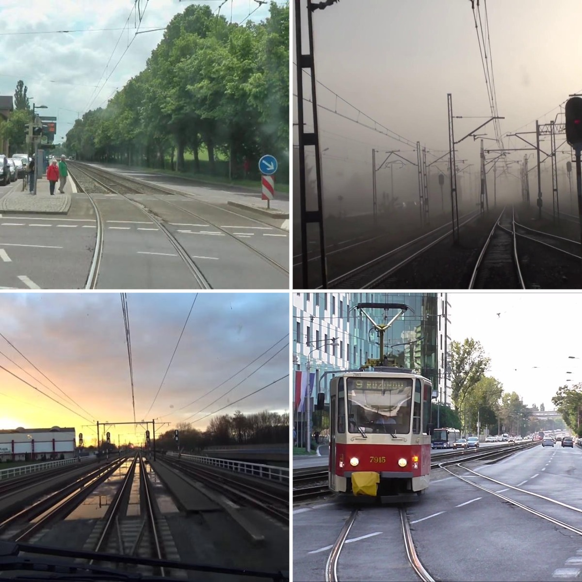
RailSem19 addresses a data gap for railway applications, offering 8,500 unique images captured from the perspective of rail vehicles, including trains and trams. The dataset features extensive semantic annotations, such as geometry-based rail-relevant polygons and dense label maps compatible with many Cityscapes road labels. A significant number of frames depict intersection areas between road and rail vehicles, such as railway crossings and trams on city streets, making RailSem19 a valuable resmyce for both rail and road applications. Due to computational resmyce limitations, My study employs a subset consisting of 2,831 images from this dataset.
Experiment
My experimental procedure begins with the detection of relationships in images, followed by the output of general risk scores using the fundamental risk analysis model I designed. It is important to note that the model produces general risk scores on a scale from 0 to 10, whereas the dataset labels indicate risk values of 0, 1, or 2. Consequently, I normalize the risk scores to these categorical values to compute accuracy.
To determine the appropriate thresholds for normalization, I computed cumulative distributions of both the labeled general risk values and the model-derived 0-10 scores. The threshold criteria were set as follows: a score less than or equal to threshold 1 is categorized as class 0, a score greater than threshold 1 but less than or equal to threshold 2 is class 1, and a score above threshold 2 is class 2. Ultimately, I selected 5 and 6 as thresholds for the RelTR model and 4.33 and 6 for the MOTIFS-SGDet-TDE model.
Results
In the comparative performance analysis, the RelTR and MOTIFS-SGDet-TDE models were evaluated based on their ability to accurately predict general risk scores on the RailSem19 dataset. The accuracy of each model was determined by comparing the normalized risk scores produced by my fundamental risk analysis model against the annotated general risk scores in the dataset. The following table summarizes the accuracy obtained for each model:
| Model | Accuracy |
|---|---|
| RelTR | 0.526 |
| MOTIFS-SGDet-TDE | 0.592 |
The MOTIFS-SGDet-TDE model demonstrates a higher accuracy (59.2%) compared to the RelTR model (52.6%). This difference can be attributed to several factors inherent to the methodologies and applications of these two scene graph generation models. The MOTIFS-SGDet-TDE model, employing a two-stage process, likely benefits from its initial object detection phase, which provides a more detailed understanding of the scene. This depth enables the model to more accurately infer relationships between entities, an advantage in the complex and dynamic environments typical of rail transportation. The two-stage approach allows for the exploitation of statistical regularities in scene graphs, improving the model’s capability to predict relevant relationships and, consequently, assess risks more accurately.
Conversely, the RelTR model, with its one-stage, transformer-based approach, optimizes for efficiency and speed in scene graph generation. While this model offers significant advantages in real-time applications, the simplified process may result in a less nuanced interpretation of complex scenes, potentially affecting its overall risk assessment accuracy. However, the RelTR model’s performance remains impressive, underscoring its viability for applications where speed is paramount.
Both models’ performances are influenced by their training on the Visual Genome dataset, highlighting the challenge of transferring knowledge from urban-centric datasets to the specialized context of rail transportation. The variations in accuracy also reflect the importance of ongoing optimization and adaptation of scene graph generation models to specific application domains, such as autonomous rail systems. The results emphasize the potential of both models in contributing to the safety and reliability of autonomous train systems.
Future Work
The exploration into the capabilities of SG Benchmark for attribute detection opens a promising avenue for enhancing the precision of my risk analysis model. The discovery that the MOTIFS-SGDet-TDE model’s checkpoint, as provided by the authors, was trained with the MODEL.ATTRIBUTE_OFF option by default indicates an untapped potential for improving object recognition and scene understanding. To leverage this potential, a retraining of the model with attribute detection enabled is necessary. Although this task presents a considerable challenge, both in terms of configuration complexity and time constraints, the benefits of pursuing this enhancement are compelling. Enabling attribute detection would allow for a more nuanced understanding of the visual scene, providing insights into not just the objects and their relationships but also their attributes. This deeper level of analysis could significantly refine the accuracy of generated heatmaps, making them more reflective of the actual risks present in the environment.
Moreover, the authors’ provision of steps for training on a custom dataset presents an opportunity to tailor the object and relationship classes more closely to the specific needs of autonomous rail transportation. Customizing the model in this way could address the unique challenges and dynamics of rail environments, from distinguishing between different types of trackside equipment to understanding the significance of various weather conditions and lighting levels on visual perception and risk assessment.
Integrating additional context-specific factors, such as weather and lighting conditions, into the risk assessment model represents another critical area for future work. These environmental factors can significantly impact the operational context of autonomous rail systems, influencing the visibility and behavior of objects and thus their associated risk levels. By incorporating these elements into the model, we can enhance its predictive accuracy and operational applicability, further advancing the safety and reliability of autonomous train systems.
The combined efforts in enabling attribute detection, customizing training datasets, and integrating additional context-specific factors hold the promise of substantially advancing our understanding and management of risks in autonomous rail transportation. These endeavors will not only improve the performance and reliability of current models but also pave the way for the development of more sophisticated and accurate AI technologies for autonomous rail systems in the future.
Conclusion
This research project has laid a foundational stone in the exploration of advanced AI technologies of vision-based risk assessment model based on scene graph for enhancing the safety and reliability of autonomous train systems. Through the development and implementation of a fundamental risk analysis model, I have demonstrated the significant potential of scene graph generation methodologies in interpreting complex visual scenes for risk assessment. Despite being an initial foray into this area, the results obtained from applying the RelTR and MOTIFS-SGDet-TDE models on the RailSem19 dataset are notably impressive. These findings not only underscore the feasibility of my baseline study direction but also highlight the substantial promise it holds for future advancements in autonomous rail transportation.
The application of scene graph generation for risk analysis within the context of autonomous trains represents a novel approach to navigating the intricate dynamics of rail environments. My work has shown that even with a basic risk analysis model, it is possible to achieve meaningful insights into potential hazards, thereby paving the way for the development of more sophisticated and accurate safety mechanisms. This project’s success is a testament to the viability of integrating computer vision and scene graph to address the complex challenges inherent in autonomous rail systems, offering a glimpse into a future where such technologies play a pivotal role in ensuring public transportation safety.
As I conclude this phase of my research, it is imperative to acknowledge the invaluable support and guidance received from my supervisors, Mr. Benjamin ALLAERT and Justin BESCOP. Their expertise, insightful feedback, and unwavering encmyagement have been instrumental in navigating the complexities of this project. Their contributions went beyond mere supervision; they provided a rich smyce of inspiration and a robust framework within which this research could flmyish. I extend my deepest gratitude to them for their significant instructions and for fostering an environment conducive to exploration and innovation.
In reflecting on the jmyney of this research project, it is clear that the path forward involves continued refinement of the models, exploration of additional context-specific factors, and the pursuit of bespoke solutions tailored to the unique challenges of autonomous rail transportation. This study has laid a solid groundwork, offering direction and inspiration for future endeavors aimed at harnessing the power of scene graph to enhance the safety and efficiency of autonomous public transportation systems.
Appendix A
The following lists all entities classes that the pretrained RelTR and MOTIFS-SGDet-TDE models are capable of detecting:
airplane, animal, arm, bag, banana, basket, beach, bear, bed, bench, bike, bird, board, boat, book, boot, bottle, bowl, box, boy, branch, building, bus, cabinet, cap, car, cat, chair, child, clock, coat, counter, cow, cup, curtain, desk, dog, door, drawer, ear, elephant, engine, eye, face, fence, finger, flag, flower, food, fork, fruit, giraffe, girl, glass, glove, guy, hair, hand, handle, hat, head, helmet, hill, horse, house, jacket, jean, kid, kite, lady, lamp, laptop, leaf, leg, letter, light, logo, man, men, motorcycle, mountain, mouth, neck, nose, number, orange, pant, paper, paw, people, person, phone, pillow, pizza, plane, plant, plate, player, pole, post, pot, racket, railing, rock, roof, room, screen, seat, sheep, shelf, shirt, shoe, short, sidewalk, sign, sink, skateboard, ski, skier, sneaker, snow, sock, stand, street, surfboard, table, tail, tie, tile, tire, toilet, towel, tower, track, train, tree, truck, trunk, umbrella, vase, vegetable, vehicle, wave, wheel, window, windshield, wing, wire, woman, zebra
Appendix B
The following enumerates the relationship classes that the pretrained RelTR and MOTIFS-SGDet-TDE models can identify between objects:
above, across, against, along, and, at, attached to, behind, belonging to, between, carrying, covered in, covering, eating, flying in, for, from, growing on, hanging from, has, holding, in, in front of, laying on, looking at, lying on, made of, mounted on, near, of, on, on back of, over, painted on, parked on, part of, playing, riding, says, sitting on, standing on, to, under, using, walking in, walking on, watching, wearing, wears, with